Neighborhood-based Recommender Systems in Rel

Recommender systems are one of the most successful and widely used applications of machine learning. Their use cases span a range of industry sectors such as e-commerce, entertainment, and social media.

Recommender systems drive multiple aspects of our everyday life. For example, when a user views a book on Amazon, Amazon offers a list of recommendations offered as  “Customers Who Bought This Item Also Bought…”.

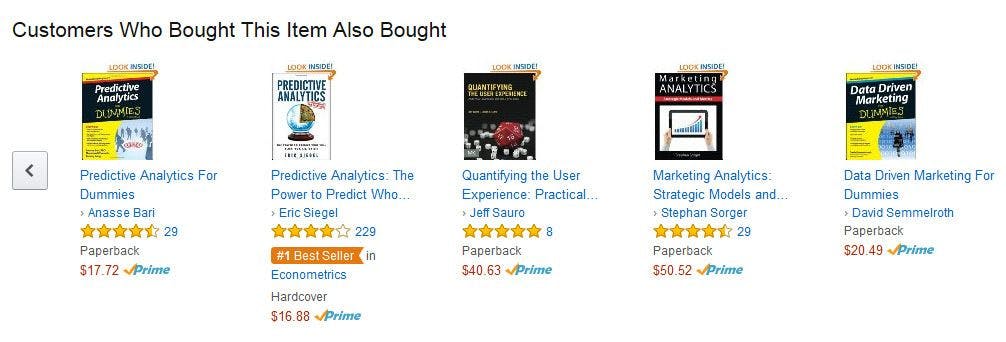
An example of a recommender system from Amazon.

In this post, we focus on a fundamental and effective classical approach to recommender systems, which is neighborhood-based.

Our Approach in a Nutshell#

Neighborhood-based recommender systems fall under the collaborative filtering umbrella and focus on using behavioral patterns, such as movies that users have watched in the past, to identify similar users (i.e., users who demonstrate similar preferences), or similar items (i.e., items that receive similar interest from the same users).

We refer to the technique that computes similar users as user-based and to the technique that focuses on computing similar items as item-based.

An example of the item-based technique is Netflix’s “Because you watched…” feature, which recommends movies or shows based on examples that users previously showed interest in.

An example of a user-based recommender system is booking.com, which recommends destinations based on the historical behavior of other users with similar travel history.

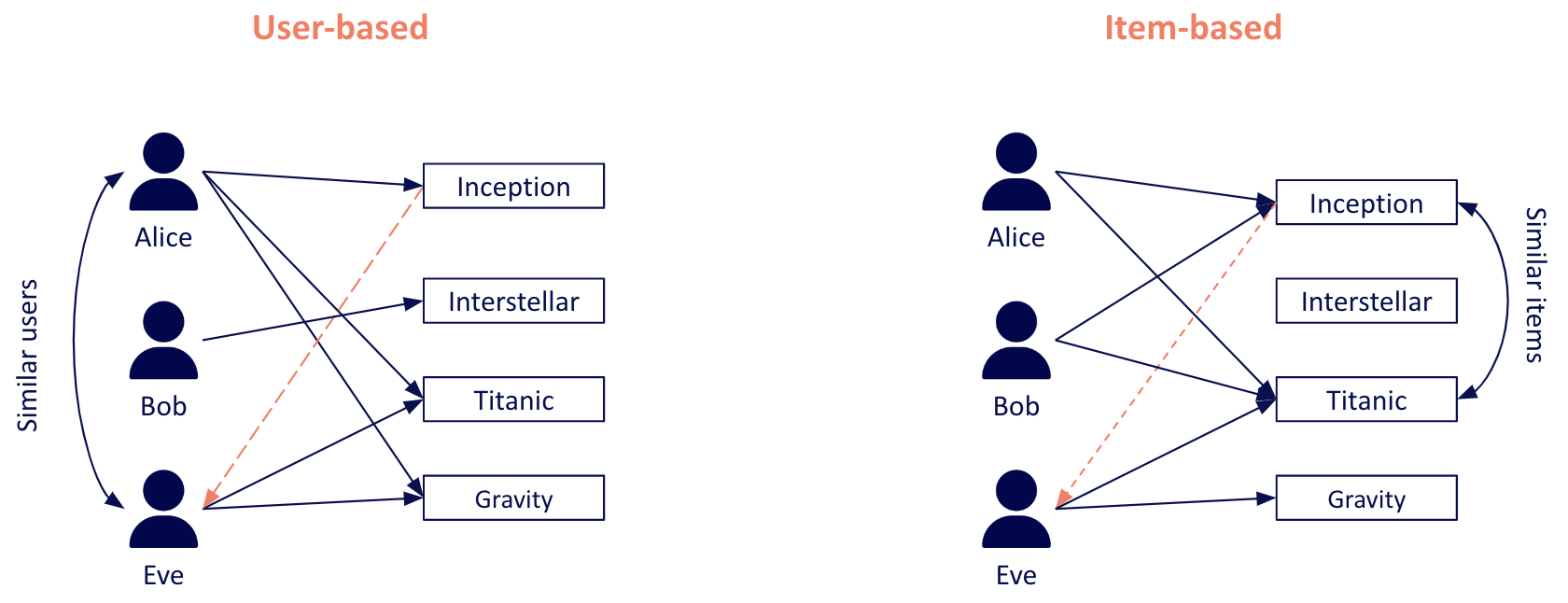
Examples of user-based and item-based approaches.

Pipeline Overview#

The image below summarizes the pipeline for our implementation of item-based and user-based recommender systems in our declarative language, Rel. Without loss of generality, we focus on a movie recommendation use case, where we are given interactions between users and movies.

• Step 1: We  convert user-item interactions to a bipartite graph.
• Step 2: We use user-item interactions to compute item-item and user-user similarities by leveraging the functions supported by the graph analytics library.
• Step 3: We use the similarities to predict the scores for all (user, movie) pairs. Each score is an indication of how likely it is for a user  to interact with a movie.
• Step 4: We sort the scores for every user in order to generate top-k recommendations.
• Step 5: We evaluate performance using evaluation metrics that are widely used for recommender systems.

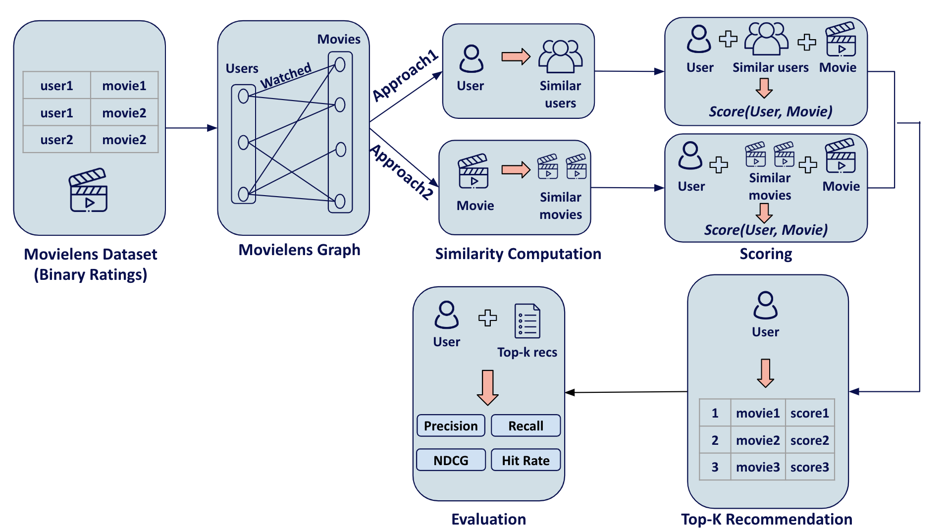
The pipeline of the neighborhood-based recommender system.

For this implementation, we use a version of the popular MovieLens100K dataset containing user-movie interactions, i.e., the presence of a (user_i, movie_i) pair means that user_i has watched movie_i.

In what follows, we cover every component of the architecture and explain how to implement it in Rel.

MovieLens Graph#

The first step is to convert the input interactions data to a bipartite graph that contains two types of nodes: Users and Movies, as shown in the image below.

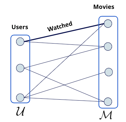
The bipartite graph representation of the MovieLens dataset.

The two node types are connected by an edge that we call watched. In Rel, Users and Movies are represented by entity types, and their attributes, such as id and name, are represented by value types.

// install
entity type Movie = Int
entity type User = Int

value type Id = Int
value type Name = String

Once we define the entity and value types, the next step is to populate the entities with data from the original MovieLens dataset.

Assuming we have a relation called watched_train(user, movie) that represents the train subset of the MovieLens data and contains the watch history for the users, and a relation called movie_info(movie, movie_name)that contains the movie names, we create the Movie entity as follows:

// update
module movie_info
 
    // entity node: Movie
    def Movie = 
        ^Movie[m : watched_train(_, m)] 
    
    // edge: has_id
    def has_id(movie, id) = 
        movie = ^Movie[m] and
        id = ^Id[m] and
        watched_train(_, m)
        from m
        
    // edge: has_name
    def has_name(movie, name) = 
        movie = ^Movie[m] and
        name = ^Name[n] and
        watched_train(_, m) and
        movie_info(m, n)
        from m,n
end
 
// store the data in the `MovieGraph` base relation
def insert:MovieGraph = movie_info 

The User entity is created similarly. Finally, we add an additional edge called watched that connects the movie entity to the user entity.

module watched_info
    //edge: watched
    def watched(user, movie) = 
        user = ^User[u] and
        movie = ^Movie[m] and
        watched_train[u, m]
        from u,m
        
    // a transposed version of `watched` to be used in the item-based approach 
    def watched_t(movie, user) = watched(user, movie)
end
 
// storing the data in the `MovieGraph` base relation
def insert:MovieGraph = watched_info

Similarity Computation#

Now that we have modeled our data as a graph, we can compute item-item and user-user similarities using the user-item interactions: movies that have been watched by the same users will have a high similarity value, while movies that have been watched by different users will have a low similarity value.

Here, we focus on the item-based method. The approach for the user-based method is very similar. There are several similarity metrics that can be used for this task. Currently, the Rel graph library provides the cosine_similarity and jaccard_similarity relations, which can be used as follows:

with MovieGraph use rated, User, Movie

def G = undirected_graph[rated]

@ondemand def L = rel:graphlib[G]

def similarities(m1, score, m2) = 
    score = L:jaccard_similarity[m1, m2] and
    // compute only movie-movie similarities
    Movie[m1] and Movie[m2] and
    // filter out self-similarities and 0 score similarities
    m1 != m2 and 
    score != 0

The relation similarities now contains movie-movie Jaccard similarity scores.

In addition to  the cosine and jaccard similarities, we can define any similarity metric. In Rel, expressing mathematical formulas is straightforward.

Here is an example defining a custom version of the dice similarity metric:

// install
@outline
module dice_similarity[shrink]
    def similarity_score[:binary, R1, R2](score)=
        n = count[x : R1(x) and R2(x)] and
        d_1 = count[x : R1(x)] and
        d_2 = count[x : R2(x)] and
        score = decimal[64, 4, n / (d_1 + d_2 + shrink + power[10, -6.0])]
        from n, d_1, d_2

    def similarity_score[:values, R1, R2](score)=
        n = sum[x : R1[x] * R2[x]] and
        d_1 = sum[x : R1[x]] and
        d_2 = sum[x : R2[x]] and
        score = decimal[64, 4, n / (d_1 + d_2 + shrink + power[10, -6.0])]
        from n, d_1, d_2
end

Scoring#

Using the similarities calculated in the previous step, we then compute the (user, movie) scores for all pairs. We predict that a user will watch movies that are similar to the movies they have watched in the past (item-based approach). 

The score for a pair (user, movie) indicates how likely it is for a user to watch a movie and is calculated as follows:

Where:

• Score_u,i is the predicted score for user u and item i
• N[i] is the set of item i’s nearest neighbors
• W[u] is the set of items watched by user u
• S_i,n is the similarity score between items i and n

In other words, the score is the sum of the similarity scores of the target movie’s nearest neighbors that have been watched by the target user.

The Rel code for the equation above is:

// install
// relation that predicts the score of a (user,movie) pair
@inline
def pred[:item_based, :binary, neighborhood_size, M, S, T](user, score, movie) = 
    score = sum[T[neighborhood_size, S][movie,n_movie] 
        for n_movie
        // the neighbor should be watched by the target user
        where  M(n_movie, user) and
	   // no score should be calculated for (user,movie) that appears in the train data
        not M(movie, user)]

The pred relation takes the following  inputs:

• neighborhood_size: The number of similar movies (neighbors) we use to predict the score
• M: The relation containing (movie, user) pairs
• S: The similarity metric, e.g., jaccard, cosine
• T: The relation that selects the top neighborhood_size most similar movies to the target movie (i.e., the nearest neighbors)

Top-k Recommendations#

To generate a list of k recommendations for a user, the last step is to rank all the scores for the particular user from highest to lowest, and then select the top k scoring movies.

Assuming we have a relation called test_items_scores(user, score, movie), we generate the top-k (where k=10 for this example) recommendations as follows:

// query
// define the size of the recommendations list
def k_recommendations = 10
// select the top k scores
def top_k_recommendations[user, rank, movie] = 
    bottom[k_recommendations, test_items_scores[user]](rank, score, movie) 
    from score

Evaluation#

To evaluate performance, we define a set of  evaluation metrics that are widely used, i.e.,: precision, recall, NDCG, and hit rate.

These metrics compute how much our recommended items overlap with the true watched items of a given user that exists in a hidden test set.

Below is the Rel code that implements precision and recall.

// install
@inline def precision_at_k[k, PREDICTED_ITEMS, TARGET_ITEMS](score) = 
    score = count[movie : PREDICTED_ITEMS(i,movie) and TARGET_ITEMS(movie) from i where i <= k] / k 

@inline def recall_at_k[k, PREDICTED_ITEMS, TARGET_ITEMS](score) = 
    score = count[movie : PREDICTED_ITEMS(i,movie) and TARGET_ITEMS(movie) from i where i <= k] / 
    count[movie : TARGET_ITEMS(movie)]

Putting It All Together#

Now that we have defined the necessary components for the neighborhood-based recommender system, let’s review a sample run that generates recommendations and evaluates them using the item-based method:

// query
with MovieGraph use watched, watched_t
with MovieGraph_test use User

def neighborhood_size = 20
def rating_type = :binary
def k_recommendations = 10
def ratings = watched_t
def approach = :item_based

def G = undirected_graph[watched]

with rel:graphlib[G] use jaccard_similarity

def sim(m1, score, m2) = 
    score =  jaccard_similarity[m1, m2] and
    Movie[m1] and Movie[m2] and
    m1 != m2 and 
    score != 0

def item_scores = pred[approach, rating_type, neighborhood_size, ratings, sim, top_k]

def top_k_recommendations(user, rank, movie) = 
    bottom[k_recommendations, item_scores[user]](rank, score, movie) 
    from score
    
def predicted_ranking = top_k_recommendations
def target_ranking = MovieGraph_test:watched
def output = average[precision_at_k[k_recommendations, predicted_ranking[u], target_ranking[u]] <++ 0.0  for u where User[u]]

In a nutshell:

1. We set the parameters for the run: the number of neighbors, the size of the recommendations list, the similarity metric, the approach, the rating type (rating values or binary ratings), and the ratings relation that contains user-movie interactions.
2. We calculate the similarities between all items.
3. We pass the relation containing the similarities to the pred relation, which computes the predicted score for all (user, movie) pairs.
4. We select the top-k scoring movies for every user.
5. We evaluate the predictions using the precision metric.

Results and Next Steps#

For the MovieLens100K dataset, the user-based method slightly outperforms the item-based method. For k =10, we achieve a best precision score of 33.6% when using the asymmetric cosine similarity metric.

The recall score for this similarity metric is 21.2%. This result is in accordance with the literature for the neighborhood-based class of algorithms.

The whole pipeline is implemented in our Relational Knowledge Graph System (RKGS), meaning that the data does not need to leave the database at any point.  Once the pipeline is implemented, generating recommendations for users is as simple as querying the database to retrieve the top K recommendations for a particular user U.

Our next post will explain how to use Rel to implement two graph-based algorithms that slightly outperform the results of the neighborhood based methods explained here. 

Part 3 will describe how to use Rel to provide content-based and hybrid recommender systems that leverage additional information signals, such as the genre of a movie.